


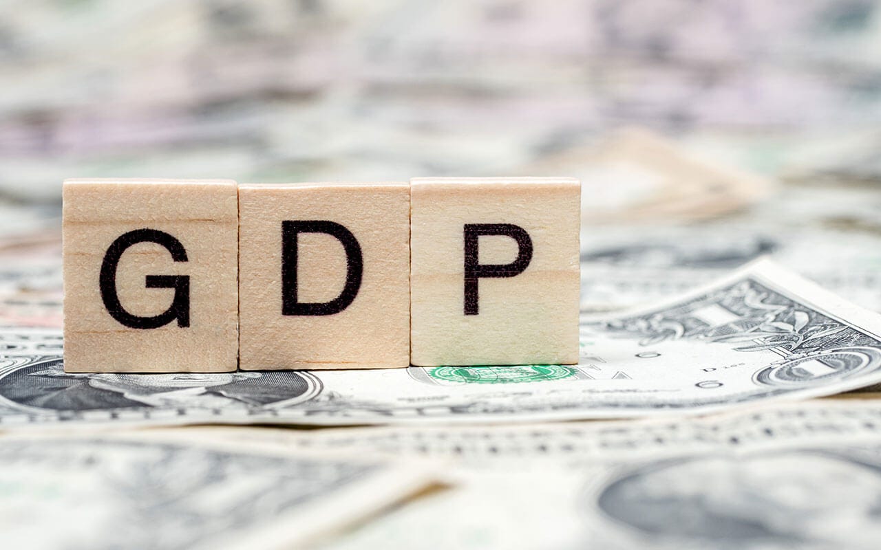
GDP Is an Important Indicator of Economic Performance, but Its Importance Has Been Exaggerated
A background piece to motivate my series on alternative approaches to economic policymaking

I got an excellent request from a reader on Monday, which was to write about how a doughnut economy or an Earth4All approach to economics could work in Canada. I love that idea!
So I am currently doing research on these other approaches, including obtaining Kate Raworth’s 2017 book Doughnut Economics: Seven Ways to Think like a 21st Century Economist from my local library. But in the meantime, I think it is worthwhile to write about GDP, particularly what it is — and is not — meant to measure in economies (hint: it is not a measure of wellbeing, and that was never its intended use).
There are very important uses of this indicator, but it has been sadly abused — particularly by political leaders and pundits who do not understand it fully. So I want to get into its pros and cons today as a background into thinking about alternative approaches to economic policy.
But before I begin, if you enjoy what I write and find it valuable, please consider a paid subscription. It will help me devote more resources into what I write so it will get even better!
Also note my 2-for-1 sale on annual Substack subscriptions remains in effect until March 31, and you can learn more about it here.
Introduction
When economists examine the current state of the economy, and when we make forecasts of future economic conditions, we refer to certain variables that may not be entirely clear to the average person. For example, when an economist says Canada is in a recession because real GDP has fallen for two consecutive quarters, what does that mean? How do we measure the amount of foreign ownership of businesses in Canada, and is foreign ownership really such a bad thing? And what exactly does GDP measure? For example, is it an indicator of wellbeing?
Therefore, the purpose of this issue of my newsletter is to clarify some of the variables economists follow closely — including GDP — and to demonstrate how they are useful in answering the above questions. I will also explain the actual intended purpose of GDP and how it has become overinflated in importance — so much so that world governments have been caught falsifying data to meet certain goals based on it, for example Greece in 2000. Indeed, I will explain drawbacks of GDP in matters such as the environment, happiness, and economic inequalities.
With these goals in mind, I will continue this post by examining how national income is measured, where I answer the following questions:
Why must an economy’s total income equal its total expenditure?
How do we define and calculate Gross Domestic Product (GDP)?
What are some alternative measures of national income?
What are the four major components of GDP?
How do real GDP and nominal GDP differ, and what is the GDP deflator?
Should we care about foreign ownership in Canada?
What are some flaws with GDP, and why is it still valuable to economists?
Why Must Income Equal Expenditure?
The typical measure of national income used by economists is Gross Domestic Product (GDP): the total income of everyone in the economy as well as total expenditures on the economy’s output of goods and services. As this definition implies, it is necessarily true that income and expenditures are identical in any economy, whether we are talking about a city, province, country, or the world as a whole. This fact is demonstrated in Figure 1 below with the Circular Flow Diagram.1

We can see there are two groups in an economy: households and firms. Also, these two groups meet in two kinds of markets:
Markets for goods and services, such as Safeway, Wal-Mart, educational institutions, and hospitals); and
Markets for factors of production, such as labour markets.
If we look at the diagram from the perspective of the “flow of inputs and outputs”, then we see that whenever a firm — such as a farmer or a provider of educational services — sells something in a market for goods and services, what they sell is necessarily bought by households; in other words, every seller must have a buyer.
Similarly, if a household offers its labour, land or capital to a market for factors of production, then those factors of production must be purchased by firms; again, every seller must have a buyer.
If we now look at the diagram from the perspective of the “flow of dollars”, we see all revenue earned by firms must also be spent by households; the revenues have to come from somewhere, and they come from household spending. Similarly, all money paid by firms in the form of wages, rent and profits must go to households in the form of income; after all, household income does not fall out of the sky.
Despite the above logic, you might still be skeptical of the simplicity of this diagram. You might argue an economy is more complicated than seen in Figure 1 because:
Households do not spend all of their income; some of it is taxed and saved.
Households also do not buy all of the goods and services in the economy; some goods and services are purchased by either a domestic government or other firms.
The above diagram also ignores trade with other countries.
You would certainly be correct to make such arguments. Nonetheless, even if we created a more complicated diagram that added more boxes — such as ones for governments and foreign countries — our conclusion does not change:
All transactions must have a buyer and a seller, so income must equal expenditures.
History of GDP as an Economic Indicator
In her book titled GDP: A Brief but Affectionate History published in 2015, Diane Coyle provides a very interesting history of GDP. I highly recommend reading this book from cover to cover.
In this history, Coyle explains that going back to the early 18th century, the economy was viewed almost entirely as restricted to the private sector, so much so that the government was hardly considered as being part of it. In fact, there was very little in the way of government policies to stabilize economies because they were not really seen as having any such role. Instead, the “classical” and economists viewed the economy in terms of Adam Smith’s “Invisible Hand”, whereby governments were to just stay out of the way and let the economy work itself out, for better or worse.
But then the Great Depression came along in 1929, and Franklin D. Roosevelt was elected President of the United States in 1932. It seemed to everyone by that point the economy might never recover, so FDR wanted a clearer picture of the state of the economy. Enter future Economics Nobel laureate, Simon Kuznets.
But going back a little further, during the 1920s-30s, Colin Clark developed methods of calculating income and expenditures in the U.K. on a quarterly basis and also adjusting them for inflation, and looking at income distributions. Clark’s work was influential to Kuznets, who applied these methods to the U.S. economy.
Keep in mind that prior to the election of Roosevelt, Coyle writes that President Hoover’s data was limited to industrial statistics such as share price indexes and freight car loadings, so they really told policymakers nothing. Therefore, when Kuznets was able to show that national income had been cut in half between 1929-32, he made a massive difference in the scope of policy, and helped FDR in his Recovery Program.
However, Kuznets did not just want to estimate national output measurements, but also national welfare (wellbeing) ones, something which GDP does not set out to measure. More specifically, he wanted to follow the lead of classical economists like Adam Smith by taking national income and then subtracting “dis-services” such as expenses on armaments, advertising, financial speculation, and — most importantly — outlays like subways and “expensive housing”. These were to be subtracted from national income because such things were viewed by Kuznets as “an evil necessary in order to be able to make a living”, rather than ends in themselves.
The problem for Kuznets was those in power viewed subtracting disservices as a peacetime “luxury”. They did not want to deduct them because if private output available for consumption fell due to the war effort, then the economy would be seen as shrinking even if government spending on the war expanded output elsewhere in the economy. Indeed, Coyle tells us the Office of Price Administration and Civilian Supply — established in 1941 — had its recommendation to increase government spending rejected on this basis.
Therefore, the Gross National Product (GNP) indicator was adopted by policymakers to overcome this hurdle. Kuznets did not like it — nope, not one bit — because GNP permitted economists to see the economy’s potential for war production, and it also ensured fiscal spending would increase measured economic growth whether or not it increased individual welfare. But he was outvoted by the “wartime realpolitik”, as Coyle put it, and government operations became significant in calculations of income.
Not long afterward, John Maynard Keynes developed GDP which included not only consumption, investment, and net exports, but also government spending, and that replaced GNP as the go-to economic indicator. In fact, Keynes basically invented macroeconomics, and Keynesian macroeconomics became the dominant economic school of thought in the post-war world.
This increased importance of government in the output statistics — beginning during the Victorian era — makes sense if one views the change in terms of monarchies in the 18th century vs. democratically-elected governments. Specifically, the monarchs back in the day did not request the consent of the people when taxing them for war efforts, so any spending by the monarchs was seen as disservices. But democratically-elected governments are — at least in theory — doing what the people want, so they are offering legitimate services that should be measured in the output statistics.
In the end, it is important to stress that GDP is an abstract idea — an empirical construct — which does not actually exist anywhere in the real world. As Economics Nobel laureate Richard Stone wrote:
To ascertain income it is necessary to set up a theory from which income is derived as a concept by postulation and then associate this concept with a certain set of primary facts.
As for the definition of GDP, it has become very complicated so I will show simplified calculations, as well as those for alternative economic indicators of national income and output.
Defining and Measuring GDP
Gross Domestic Product (GDP) can be defined as the market value of all final goods and services produced within a country in a given period of time. For greater clarity, in their Principles of Macroeconomics (Canadian Edition) textbook, Mankiw, Kneebone, and McKenzie (2011, pp. 100-103) divide this definition into several parts:
“…the market value…”: we use the prices that are actually charged for goods and services when we calculate GDP. This is logical as governments are likely in no position to measure the true value of every good and service sold in the economy.
“…of all…”: even if something does not have an explicit market rate, its market value is estimated, such as owner-occupied housing where governments assume owners pays rent to themselves. Exceptions to this rule include illegal activities and stuff not sold in markets — such as household operations like cooking, cleaning, and taking care of one’s own kids.
“…final goods and services…”: GDP does not count intermediate goods, which are goods that are used as inputs to create something else, which is then sold to a final consumer. Exceptions to this rule include stuff that is kept in inventory until later; they are then counted as negative inventory when sold.
“…produced…”: GDP excludes goods and services produced in past periods, such as used cars and goods that were held in inventory from previous periods. We exclude such goods and services from the calculations as they were included in GDP when they were originally produced; to include them again would result in double-counting over time. But if resold after making improvements, then only the value-added is included.
“…within a country…”: we only include goods and services produced in the country in question, regardless of the nationality of the producer.
“…in a given period of time”: GDP is usually calculated by year or quarter. The time period used by economists depends on the purpose of the data. For example, if we are determining whether we are in a recession, we use quarterly data because a recession can be defined as two consecutive quarters of negative real GDP growth; if we want to compare growth rates across countries or over long periods of time, then annual data will likely be sufficient for our analysis.
As demonstrated using the Circular Flow Diagram in Figure 1, we can calculate GDP using either the income or expenditure.
The income approach is summarized as follows:
GDP = wages, salaries, and supplemental labour income + interest and miscellaneous investment + net farm income + net income to unincorporated businesses (UBI) + corporate profits (before tax) + government business enterprise profits + indirect taxes less subsidies (included because they are levied on currently produced stuff, and are not included in wages like income and corporate taxes) + depreciation (“capital consumption allowance”)
where:
Corporate profits (before tax) = dividends + retained earnings + corporate tax
Other Measures of National Income
Economists also make use of several other measures of national income, including the following ones:
Gross National Product (GNP): total income earned by a nation’s permanent residents, regardless of where they were located when they earned the income. It does not include income earned in Canada by foreign nationals. Usually GNP and GDP are very close to the same value.
Net Domestic Income (NDY): the value of GDP after taking into account the loss in value of capital, as well as transfers between businesses and government:
NDY = GDP - depreciation - indirect business taxes + business subsidies
Depreciation is also known as capital consumption allowance, while an example of indirect business taxes is sales taxes. NDY accounts for capital consumed over the year, and thus estimates how much a country would need to spend to maintain its current GDP.
Personal Income (PY): income households and non-corporate businesses earn from all sources:
PY = NDY - corporate profits (before tax) - government business enterprise profits + dividends + income from government transfer programs
Income from government transfer programs includes EI, CPP, and welfare.
Personal Disposable Income (PDY): personal income households and non-corporate businesses have left after satisfying government obligations, such as taxes, and traffic tickets:
PDY = PY - personal taxes
An equivalent definition of personal disposable income takes into account that whatever income is not spent must be saved:
PDY = Personal Saving (S) + Consumption (C)
Combining these two definitions, we can then redefine personal income as:
PY = C + S + personal taxes
Note it is possible for personal saving (S) to be negative, which would imply we are borrowing money to finance our consumption spending. Thus, it is useful to define the break-even level of income as the amount of income we would need to earn, so we can pay for everything we want (or need) to consume without borrowing anything — so S = 0, meaning PY = C.
To apply what we just learned, suppose we have the following consumption function:
C = 490 + 0.7Y
where Y ≡ PY = PDY for simplicity (so no taxes). Please answer the following:
If Y = 490, what is C? What is S?
C = 490 + 0.7*490 = 833
Thus:
S = Y - C = 490 - 833 = -343
What is the break-even level of income? It is where Y = C so set:
Y = 490 + 0.7Y → 0.3Y = 490 → Y = $1,633.33
As if the above definitions of income were not exciting enough, there is another one:
National product: the value of a national economy’s total production of goods and services. Really, this is just another way of saying “national income”, which itself is usually measured by GDP (as explained above).
For practice, please answer the following question: suppose Appliance Mart buys a used fridge for $100, repairs it, and resells it for $250. How much will this transaction change national product, if at all?
It will increase it by:
$250 – 100 = $150
That is because it is the value-added of the repairs. If the original new price was $500, then we would not count the depreciation because we count gross investment; but we would still count $150 value added because it is new production.
Moving on, one of the most important uses of GDP is to examine how strong or weak the economy is performing at a given time, or over time. Thus, economists define the output gap as the difference between actual output and potential output.
In this definition, actual output (Y) is what we use to measure GDP, but potential output (Y*) represents what our economy could produce if it was operating at full employment — basically meaning everyone who wants a job has one.
When we are not at full employment, the output gap is:
An inflationary gap when Y > Y*
A recessionary gap when Y < Y*
To help you understand the meaning of an output gap more clearly, I have used the information provided in Table 1 below to calculate the output gap for each year.

In summary, several measures of national income are used by economists to examine the economy, but they all tend to tell the same story: if GDP is growing (falling) rapidly, then these other income measures are also growing (falling) rapidly. Thus, when monitoring fluctuations in the overall economy, it matters little which measure of income is used.
Components of GDP
The more useful method to define GDP when teaching economics is the expenditure approach. This approach is more useful than the income approach for our purposes, as governments use fiscal (tax-and-spend) policies to change their own spending patterns, or to motivate businesses and consumers to change their spending patterns.
Similarly, central banks — such as the Bank of Canada and the U.S. Federal Reserve — use monetary policies to change the money supply by motivating consumers and businesses to modify their spending patterns.
Therefore, I will now divide GDP into its four expenditure components:
Y ≡ C + I + G + NX
where:
Y = GDP
Consumption (C) includes spending by households on goods and services, which includes postsecondary education spending.
Investment (I) includes the purchase of goods and services by businesses that will be used to produce more goods and services. More specifically, it is the sum of purchases of capital equipment, inventories, and structures. Furthermore:
Gross investment = net investment + depreciation
What is not considered investment? Used housing or financial investments because nothing is produced in the current period — interest on financial investments is counted indirectly when spent on C, I, G or NX.
.
What if a firm keeps investment in inventory, and then resells it later? It is then counted as investment; when sold, it is counted as negative investment to offset the increase in C, because we want to measure current production in current GDP.
Government Spending (G) includes spending on goods and services by all levels of government. It includes salaries of government employees and spending on public works.
.
What does it not include? Transfer payments such as CPP or interest payments on government debt — again, because nothing is currently being produced as opposed to spending on health and education which go into new production.
Net Exports (NX) is the difference between how much Canada sells/exports (X) to foreign countries, and how much it purchases/imports (M) from them:
NX = X - M
Imports are subtracted from the equation to cancel out their effects on other components of GDP, since we only want to include domestically produced goods in GDP. For example, if a household imports a Volkswagen for its own personal use — meaning it is not resold — then this transaction will raise both C and M and therefore there is no overall effect on GDP.
Note this GDP equation is an identity because the two sides of the equation must always be equal: every dollar of expenditure included in GDP must fall under one of the four right-hand side categories.
Furthermore, if we want to focus only on how much is being spent by Canadians on goods and services, whether they are governments, consumers or businesses, then we can calculate Final Domestic Demand (FDD):
FDD = GDP - NX
Given the importance of the above definition of GDP, please consider the following transactions and identify whether C, I, G, or NX will rise, as well as whether will GDP rise. Assume we are calculating Canadian GDP, unless otherwise noted.
Purchase of earthmoving equipment from China by a Canadian corporation. I, because it is investment by a Canadian corporation, but since GDP only measures domestic production, it also raises M, thus lowering NX by the same amount.
Your Canadian grandmother receives a pension. None, because it is a transfer payment which does not reflect current production or G, since the government took it from past periods.
You buy an Italian sports car. C and M, cancelling each other out.
Suncor buys domestically produced equipment. I and GDP rise.
You buy stocks. None, because saving does not reflect current production — I will eventually rise since I = S, but there is no direct effect of saving on GDP.
The BC lumber industry sells $100,000 in lumber to China; in the same period, the Canadian government buys $150,000 in wooden office furniture from China. X rises by $100,000, followed by a rise in both M and G of $150,000 each. Since imports are not produced here, the value of M is cancelled out and only the Canadian value-added of $100,000 is counted in GDP in the end — which shows why higher imports cannot lower our GDP, because they are always completely offset, and often more so if value-added, by increases in C, I, G or X.
Singapore imports $10,000 in clothing, re-labels that clothing and then exports it for $10,500 in the same period (so we focus on Singapore’s GDP equation). M will rise by $10,000 but nothing else yet, because it is not sold to a final consumer; then X will rise by $10,500 so Singapore’s GDP rises overall by $500 — just the value-added.
A Canadian engine manufacturer sells an engine to a Canadian automotive manufacturer for $3,000; the engine is then placed into a car which is sold to a household for $30,000 in the same period. The original $3,000 does not count at all because it was never sold to a final consumer — unlike an export which can be considered to be sold to a final consumer from a Canadian perspective. The final car sale then raises C and GDP by $30,000, so no double-counting of the engine.
You earn $1,500 in capital gains on a financial investment, which you spend on a new personal computer in the same period. The capital gains do not affect anything in GDP because it does not reflect current production, but when you spend these capital gains it will raise C by $1,500 and thus raise GDP by $1,500.
Real vs. Nominal GDP
Now that we understand how to define and calculate GDP, suppose we want to track the Canadian standard of living (per-capita GDP) over time. If we do not adjust for inflation, then we cannot be certain whether an increase in GDP is due to an increase in the economy’s standard of living, or simply due to rising prices.
Therefore, we need to distinguish between two types of GDP:
Nominal GDP: the market value of all final goods and services produced within a country in a given period of time, measured in current dollars.
Real GDP: the market value of all final goods and services produced within a country in a given period of time, measured in some base year’s dollars.
I will now show how to calculate nominal GDP and real GDP using the following example in which an economy produces three goods: back bacon, beer and toques. Quantities and prices per unit for years 2023 and 2024 are provided in Table 2:

I will now answer the following questions:2
What is nominal GDP in each of 2023 and 2024? By what percentage does nominal GDP change from 2023 to 2024?
Nominal GDP (2023) = 500*4 + 1,000*24 + 1,700*5 = 34,500
Nominal GDP (2024) = 700*5 + 2,000*30 + 3,000*7 = 84,500
Growth Rate = [(84,500 – 34,500) / 34,500] * 100 = 144.9%
Using prices for 2023 as the set of common prices, what is real GDP in each of 2023 and 2024? By what percentage does real GDP change from 2023 to 2024?
Real GDP (2023) = 500*4 + 1,000*24 + 1,700*5 = 34,500
Real GDP (2024) = 700*4 + 2,000*24 + 3,000*5 = 65,800
Growth Rate = [(65,800 – 34,500) / 34,500] * 100 = 90.7%
Using prices for 2024 as the set of common prices, what is real GDP in each of 2023 and 2024? By what percentage does real GDP change from 2023 to 2024?
Real GDP (2023) = 500*5 + 1,000*30 + 1,700*7 = 44,400
Real GDP (2024) = 700*5 + 2,000*30 + 3,000*7 = 84,500
Growth Rate = [(84,500 – 44,400) / 44,400] * 100 = 90.3%
Why are the two output growth rates constructed in 2. and 3. different? Which one is correct?
.
The answers measure real GDP growth in different units. Neither answer is incorrect, just as a measurement in inches is not more-or-less correct than measurement in centimetres — but if we change basket of goods, the base year should use the most recent basket of goods so that we have prices for all goods in that basket, because if use the previous year, then the price will be zero for some goods. Otherwise, what really matters is we are consistent so comparisons over time or across countries/regions are consistent.
To summarize:
Nominal GDP = Sum of total revenue for each good using current prices
Real GDP = Sum of total revenue for each good using base-year prices
In both cases, we use monetary values because we cannot sum apples and oranges, but we can sum the values of apples and oranges.
It is important to remember that if economists refer to GDP, we usually mean real GDP because we want to exclude the effects of inflation. Also, when we talk about growth, we are referring to percentage changes in real GDP over time.

We can now use both nominal and to compute a third statistic:
GDP Deflator = (Nominal GDP / Real GDP) * 100
Real GDP reflects changes in productivity but not prices, but the GDP deflator reflects changes in prices but not productivity. Thus, the latter indicator is a measure of inflation.
Application: returning to our example in Table 2, compute the GDP deflator for each of 2023 and 2024, using 2023 as the base year.
2023 GDP Deflator (2023 dollars) = 34,500 / 34,500 * 100 = 100.0
2024 GDP Deflator (2023 dollars) = 84,500 / 65,800 * 100 = 128.4
So prices rose by 28.4% between 2023 and 2024, and this rise had nothing to do with productivity — it is all inflation. In other words, the 144.9% growth in nominal GDP is due to 90.7% growth in productivity (real GDP) and 28.4% price inflation.
For realistically small changes in P and Q, both percentages add up almost perfectly to nominal GDP growth, but technically there is a multiplicative factor so the other 25.8% = 90.7% * 28.4% represents combined productivity and inflation changes.
Foreign Ownership and the “Hollowing Out” of Canadian Industry
Earlier in this post, I defined GNP and GDP as follows:
GNP measures the value of all income earned by domestic nationals (Canadians), regardless of where it is earned.
GDP is the value of all income earned domestically (in Canada), regardless of the nationalities of the people who earned it.
Also, (GNP - GDP) measures the difference between the value of output produced here by foreigners, and the value of output produced by Canadians in foreign lands. This difference rises in size as people in other countries purchase more of Canada’s productive capacity, and as Canadians purchase less production of other countries.
In the 1970s, many people in Canada became concerned as the size of this difference grew larger. This growth was interpreted as evidence that Canada was being “hollowed out”. This fear prompted the federal government to impose controls on foreign ownership, such as by passing the Foreign Investment Review Act (FIRA) in 1974. It was designed to monitor and regulate the purchase of Canada’s productive capacity by foreigners. FIRA was repealed in 1985.
The (GDP – GNP) figure continued to grow as a proportion of GDP until the 1980s when it levelled off at 3.5% of GDP. Since 1999, this proportion has fallen significantly, and returned to 1960s levels in 2005.
This gap partly reflects the relative attractiveness of Canada as a place to produce goods and services: it mirrors movements in the prices of commodities that Canada produces abundantly (oil, gas, nickel, uranium). During the 1980s and 1990s when commodity prices were lower, other countries were viewed as more attractive places to invest. After 2000, this opinion reversed as commodity prices rose.
Problems with Cross-Country Comparisons
Once again, Coyle goes into much more detail on these problems, and I recommend reading that book from cover to cover. I will briefly summarize her points here.
There are problems with comparing GDP statistics across countries, particularly when comparing developed countries to developing countries, and that is partly in how we actually make these comparisons.
For example, one way is to do so is to use exchange rates to convert all statistics into the same currency, but there are countries where exchange rates are not market-based; they are fixed (or managed) by their governments/central banks. Therefore, these exchange rates do not truly reflect relative purchasing power.
Even when exchange rates are flexible, they can fluctuate wildly due to whims of financial markets that are not always economically logical — think of GameStop in terms of stock markets.
Then there are non-tradables like services which are not measured in foreign exchange markets like haircuts, healthcare, and education — which are very cheap in lower-income countries — so using market exchange rates to compare GDP in lower-income countries with low trade volumes to higher-income countries with high trade volumes is biased.
Therefore, we want to take relative purchasing power and living standards into account when comparing GDP across countries, so economists use Purchasing Power Parity (PPP) exchange rates to adjust GDPs — the Penn World Tables being the primary example which many economists use. Most growth studies use them, as do policymakers in national governments and international agencies.
The problem is these PPP rates raise the GDPs of low-income countries which have a lot of cheap non-tradables; indeed, that is the point of using them, but research shows it actually overestimates GDP, and thus understates differences in living standards. That in turn makes it harder for them to get loans from the World Bank, for example, which motivated China to convince the World Bank to reduce its estimates of GDP per capita in 2000.
It is also a problem to use PPP because lower-income countries have quite inferior statistical agencies, so they do not measure the relevant statistics well compared to developed countries. Some countries also sometimes flat-out refuse cooperation, like China and India.
Finally, Coyle points out there is an unconscious ideological bias because statistics show inequality and poverty worldwide going down, which puts more confidence in standard globalist trade and investment policies. Obviously, we can see just by looking with our eyes at China that living standards have improved there, but it can still be overestimated when converting GDP figures using PPP.
Historical Events Raising Doubts About GDP
After WWII, Coyle explains why it seemed the good times would never end, and there were good reasons for that expectation. For example:
There were impressive technological improvements which makes capital and labour more productive.
The labour force became increasingly educated, and this increased education also led to the development of better capital.
There was increased military innovation such as synthetic rubbers and plastics.
There were significant improvements in air travel, radio communications, and personal computing, for example.
With the help of the introduction of credit cards, mass consumerism became a thing, which involved increased consumption due to an increased availability of consumer goods, which in turn increased employment and wages.
Having more time to relax and enjoy life due to the increased prominence of automobiles, phones, refrigerators, and washing machines, also led to the “invention” of teenagers in the 1950s. With this increased relaxation time, there was also increased demand for TVs, radios, cameras, fashion, and music.
The good times also led to healthcare improvements such as vaccinations.
Therefore, everything seemed groovy, where a family of four could afford a very, very, very fine house with two cats in the yard, all on just one income to support the entire family. If the economy started declining, the government would use its Keynesian policy tools to stimulate it back to its previous strength.
And even though all of this stimulation led to more inflation, that was fine because the Phillips Curve tradeoff between inflation and unemployment meant higher inflation was correlated with lower unemployment. Unions could fairly easily demand higher wages to offset the negative effects of inflation, so no one had any complaints.
But as Coyle argues, things were actually too good and there was too much growth. She provides four reasons why previous economic wisdom crumbled in the 1970s, followed by more reasons in the decades that followed.
1970s Stagflation
First, policymakers failed to realize the growth they were “creating” was by design because GDP is constructed to rise as government spending rises. But eventually OPEC got its oily hands into the machine by reducing its supply of oil to world markets, which created something no one ever expected: stagflation, which is where there is both increased unemployment and increased inflation at the same time!
Therefore, when governments tried to stimulate the economy in exchange for increased inflation using the old Phillips Curve logic, it did not work so well. And that helped right-wing governments come into power by the early 1980s — including Margaret Thatcher in the U.K. and Ronald Reagan in the U.S. — who turned against Keynesian economic policies and became more enamoured with deregulation, low taxes, privatization, and tight monetary policy.
The Fall of Communism
Then there was the realization that communist countries like the USSR and China were not as well-off as they let on. In the early decades of the Cold War, very few Westerners had stepped foot into these countries, so even learned experts believed their falsified economic statistics.
The veil was lifted by the 1970s, but before that happened, people in the West were getting sick of 20 years of living with the Cold War, which included the Vietnam war. And given their belief that life was already much better in the Communist countries, stagflation intensified their anger that already led to civil rights protests and strikes.
By the time everyone realized Communism was not such a utopia, it was too late: Reagan and Thatcher powered up and put more limits on these protests and strikes.
Environmentalism
Then there was the environment, something which is not reflected in GDP because it is not part of the market system.
People in general were ecstatic with the growth happening in the economy, but now some of them started worrying about the effects of growth on the environment, particularly after seeing the Earth from space. As a result, the Club of Rome published The Limits to Growth, while Paul Ehrlich published The Population Bomb where he predicted millions of people would die during the 1970s — extended to the 1980s in later editions when these deaths did not happen.
Ehrlich’s mistake was not taking seriously the economic fact that the price of things rise when they become scarcer, so people would reduce their consumption as prices rise. But that does not mean the environment is not important, because it very much is (increasingly) so!
In fact, there are economists whose entire careers are devoted to environmental economics and who do care more about climate change than economic growth, despite what people like David Suzuki think.3
And that is why most economists prefer carbon taxes as an approach to fight climate change: these taxes push and shove the environment into the market system, so it is no longer what we call an “externality”.
Human Development
In the 1970s, economists found that according to GDP per capita figures, high-income countries had massive growth, but not so much the lower-income ones. They also wondered whether GDP per capita the best indicator for cross-country comparisons.
Well, Coyle tells us that Mahbub Ul Haq — a Pakistani economist working at World Bank in 1970s and 80s — developed the Human Development Index (HDI) to measure poverty and welfare, which measured capabilities instead of income. It was also based on work by Economics Nobel laureate Amartya Sen who argued (as written by Coyle):
…famines had nothing to do with income and poverty; rather they were caused when governments were not responsive to the needs to their people, and in particular when there were no newspapers or broadcasters with sufficient independence to challenge and criticize government decisions. Democracies did not suffer famines at any level of GDP per capita.
He also said income per capita was important, but not as a complete measure of people’s welfare as their capabilities — including health education, women’s freedom, infant mortality, life expectancy, and access to key technologies like electricity and roads. The HDI measures these separate indicators and combines them into a single ranking, published annually by the UN Development Program.
In her book, Coyle writes that high GDP per capita countries are also often at the top for HDI, and vice versa, but not always: at the time of writing, the U.K. was high in GDP but lower in HDI. Nonetheless, there is still a positive correlation between the two, because richer countries are more able to afford these other indicators.
But it must be stressed the two indicators are still very different in the sense that HDI is a welfare measure, not an output measure.
Ironically, haters of GDP still tend to focus on poverty and income measures when looking at developing countries. But some good news is that the indicators included in the calculation of the HDI are narrowing around the world, partly due to massive foreign aid, and despite the lack of progress in terms of GDP per capita growth.
Increasing Importance of Services and Other Intangibles
By the 1990s, the tech boom was on the rise, but a problem was services, innovation, and the digital economy were becoming much more important as a result. And they are much harder to measure when estimating GDP.
For example, how do we measure the productivity of a healthcare worker? Is it by the number of patients seen? Should we only measure patient outcomes in certain ways? These cannot be definitely answered, but services account for more than two-thirds of GDP in OECD countries at the time of Coyle writing her book.
There is also the issue of measuring variety as an effect of innovation. For example, with innovation there can be significant price decreases as quality increases, but those price decreases mean GDP is being underestimating, particularly since quality is hard to measure with markets. Furthermore, there is econometric evidence that consumers value choice, but it is not measured in the GDP statistics.
These problems are especially relevant to computing technology and the Internet because prices have fallen dramatically, but their quality is so much higher, so we are better off from these technologies, but it does not show sufficiently in GDP growth.
Statistical agencies like the ones in the U.S. therefore turned to “hedonic” price indexes to convert GDP to measure these quality factors, more specifically to take into account quality changes in order to figure out the true price of the underlying benefit to the user. For example, various features of a computer were measured such as screen size, hard drive space, resolution, built-in WiFi.
But this change and others made GDP growth look a lot stronger than was the case — the economy was indeed booming, but maybe not as much as the GDP figures let on, especially since other major countries like Japan and those in Europe had not yet made the changes.
And GDP still does not account for services well, although they keep growing in importance to economies.
So while these alternative approaches are nice, the fact remains GDP measures output and production — not welfare, and therefore not quality and variety. Therefore, Coyle argues that any modifications like hedonic pricing are trying to turn it into something for which it was never intended. We need something that measures welfare.
2008 Financial Crisis
According to Coyle, the crash made economists wonder how much the finance sector has increased economic welfare at all. She goes through this issue in much more detail than I do here, but a big problem is a follows: increased risk taking is recorded in GDP figures as increased real growth in financial services. That is odd because merely taking on risk is not necessarily productive — although managing it is productive.
Overstating the contribution of risk-taking matters to us because political leaders shape policies around certain key sectors, such as regulatory reform of the financial sector. If banks appear to be contributing so much to GDP, then governments will deregulate to avoid holding them back, and that led to the crash.
But is finance productive at all? Adam Smith said “no”. GDP escapes this question because it focuses on what people pay for something — and if they pay for it, it must be productive. But of course, it also includes stuff we do not actually pay for directly, but still use, such as public services paid through taxation.
Black Market Activity (Informal Economy)
Another issue with GDP is it is difficult to include the black market economy in it because — by design — it is not open to statistical measurement by governments. Nonetheless, Italy started estimating it in 1987, which raised its GDP so much it passed the U.K. to be fifth highest in world!
The informal economy is especially large in developing countries, again showing how badly GDP is estimated there. Now a number of economies make a similar adjustment.
But GDP still does not include household production — such as cooking, cleaning, and taking care of one’s own kids — which is difficult to measure given the fact it is unpaid, although there are time-use surveys in countries like Canada.
Coyle notes some people have tried to get around this complaint by arguing home activities like childcare is both work and leisure as it is pleasurable, so it is okay to not count it in GDP. But a counterargument is a lot of people also enjoy their paid work.
GDP and Economic Welfare
As claimed earlier, GDP is considered by economists to be the best measure of economic growth in a society, even though it was never designed to actually measure wellbeing. We just focus on it because it is relatively easy to quantify and it is strongly correlated with actual indicators of wellbeing.
For example, GDP does not measure important intangibles, such as the quality of healthcare and education, the beauty of poetry, the intelligence of our public debate or the integrity of our public officials. While this is true, nations with larger GDPs can afford better healthcare and better educational systems, etc.
Nonetheless, there are still other legitimate criticisms of an overreliance on GDP as an indirect indicator of economic welfare:4
Leisure: if a person works longer hours, their extra productivity is reflected in a rising GDP. However, GDP does not reflect the reduction in that person’s leisure — the tradeoff — which would lower that person’s welfare.
It also ignores income distribution: it looks only at the average person.
Broken Window Fallacy: the belief that destruction, whether it is deliberate or due to a war or natural disaster, is good for the economy because the expenditures to rebuild it all will increase GDP. A problem with this logic is the resources put into recovery could have otherwise been put to use somewhere else.
Coyle notes it has been pointed out that at a single point in time, higher-GDP countries are happier than lower-GDP ones, but it is not true within a country over time. However, this fails to recognize that happiness has an upper bound as with life expectancy and height, but not GDP. Also, if we go the other way, then GDP falling a little can lead to happiness falling a lot.
But people still argue about the link between GDP and welfare, when there is no real link because it was never meant to measure welfare. There is a correlation, but that was not the intent. We need something else to measure welfare.
Coyle argues we should not be trying to raise GDP to raise happiness, and we should not be arguing there is a peak level of desired GDP because then we are happy enough. We need a different measure altogether. Economists know deep down this is true, but we unintentionally give the impression they are linked more than they are because we use it so much.
In the end, Coyle argues GDP is flawed but still necessary because we need a bigger economic pie to distribute more to everyone else. But it is only a measure of output, not welfare. And we still need a better measure of sustainability, meaning whether current growth limits future growth and living standards, including environmentally.
She also argues GDP is an important measure of freedom and human capability created by capitalism. It imperfectly indicates innovation and human possibilities, as well as creativity and care for one another in an economy based increasingly on intangibles and services.
She defends GDP as a key indicator for economic policy — better than some like happiness indexes. But it should not be the only indicator because it was designed in 1940s for a primarily manufacturing economy, not one of services and intangibles.
Closing Remarks
Let’s end this issue of my newsletter by summarizing the answers to the questions asked in the introduction. First, in terms of measuring national income:
Why must total income always equal total expenditure for an economy? Each transaction has a buyer and a seller, whether they involve households, business, government, or foreigners. See the Circular Flow Diagram.
How do we define and calculate GDP? We could use the income approach or the expenditure approach (Y = C + I + G + NX). They are equivalent given the fact that income must always equal expenditures.
What are some alternative measures of national income? There are several — e.g., GNP, NDY, PY, PDY, and national product — but they all generally tell the same story. We therefore tend to use GDP.
Divide GDP into its four major components: They are C, I, G, and NX.
How do real GDP and nominal GDP differ from one another, and what is the GDP deflator? Real GDP takes inflation out of the equation to create a productivity measure; the GDP deflator is an inflation-only measure.
Should we care about foreign ownership in Canada? The amount of foreign ownership in the domestic economy is measured as GDP - GNP. Many people worry a lot about the costs of foreign ownership, but we should always remember that foreign ownership does bring great benefits to Canadians.
Identify some flaws with the GDP measure, and explain why GDP is still a good indicator of economic welfare: It excludes several important variables, but it is still an excellent indicator of economic welfare, even if only indirectly. Nonetheless, we should not rely on it too much as an indicator of wellbeing; we need to have other tools in our toolbox for that purpose.
Thank you for reading to the end. If you like what you see and want to support me with a paid subscription, please do not restrain when you hit the following “subscribe” button! Regardless, I am glad you are here. I hope you have a great day!
Source: Mankiw, N. Gregory, Ronald D. Kneebone, and Kenneth J. McKenzie (2011). Principles of Macroeconomics, Fifth Canadian Edition. Toronto: Thomson-Nelson, page 25.
Note the calculated growth rates are ridiculously unrealistic, but I chose these numbers for the purposes of clearly differentiating the effects of inflation vs. productivity on growth.
As explained by Canadian economist Chris Auld, while a university student David Suzuki took an Economics class, and during the first lecture, the professor taught the Circular Flow Diagram. Suzuki asked where the environment fit into the diagram, and the professor responded it was not in there, because it is an “externality”. Rather than ask for clarification, Suzuki walked out and has been (wrongly) telling everyone since then that “We don’t give a shit” about the environment. For more on David Suzuki’s willing ignorance of economics, see Mike Moffatt here and here.
One economist who has become very frustrated with the common misperception that economists only care about GDP is Andrew Leach.